Computational Fluid Dynamics: 9 Powerful Steps Explained

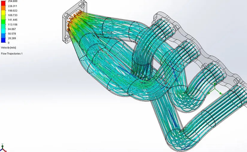
Computational fluid dynamics (CFD) uses numerical methods and computers to predict how liquids, gases, heat, and related physical quantities behave inside or around a defined geometry. Engineers use computational fluid dynamics to study airflow over vehicles, pressure loss in pipes, temperature distribution in electronics, combustion inside furnaces, ventilation in buildings, and many other systems that would be difficult, expensive, or unsafe to investigate through physical testing alone.

A CFD result is not automatically correct because it looks realistic. Its credibility depends on the question, geometry, equations, assumptions, mesh, boundary conditions, numerical settings, convergence, verification, validation, and uncertainty. This guide explains the complete workflow in plain language. For a broader view of simulation, manufacturing, thermal systems, and digital engineering, visit our engineering and manufacturing guide.

What Is Computational Fluid Dynamics?

Computational fluid dynamics is a branch of engineering analysis that divides a flow domain into many small cells or elements and solves approximate forms of governing equations across them. The equations represent conservation of mass, momentum, and energy. Depending on the application, a model may also include turbulence, species transport, chemical reactions, radiation, phase change, particles, porous media, rotating equipment, or interaction with solid structures.

The output may include velocity, pressure, temperature, density, turbulence quantities, heat-transfer rate, forces, mixing, concentration, residence time, or other variables. Engineers convert those fields into decisions: whether a fan is large enough, a component will overheat, a pressure drop is acceptable, a wing produces the required lift, or a process distributes material uniformly.

How Computational Fluid Dynamics Works

Fluid behavior is governed by mathematical relationships that are often too complex to solve exactly for real geometries. Computational fluid dynamics transforms those continuous equations into algebraic equations at discrete locations. A solver repeatedly updates the variables until the numerical solution meets defined convergence criteria.

This process introduces approximations. Geometry may be simplified, a mesh cannot contain infinitely small cells, turbulence is modeled, and boundary conditions represent the surrounding system with limited data. Good CFD practice manages these approximations and demonstrates that they are suitable for the intended decision.

The Three Foundations of a CFD Model

Conservation of Mass

Mass cannot appear or disappear inside an ordinary flow model. For steady flow through a pipe without leaks or accumulation, the mass flow entering should equal the mass flow leaving. Continuity provides an important consistency check in computational fluid dynamics results.

Conservation of Momentum

Momentum equations connect fluid acceleration with pressure, viscosity, gravity, and other forces. They help predict velocity, pressure distribution, drag, lift, recirculation, jets, and separation. The well-known Navier–Stokes equations describe these relationships for many fluid problems.

Conservation of Energy

Energy equations represent heat transfer, work, and temperature change. They are essential when computational fluid dynamics is used for heat exchangers, electronics cooling, combustion, HVAC, turbines, furnaces, or any process where temperature affects performance.

9 Powerful Steps in the Computational Fluid Dynamics Workflow

1. Define the Engineering Question

Begin with a measurable decision, not a request for colorful images. Define the output, operating range, acceptable uncertainty, timeline, and consequence of error. A question such as “Which duct design keeps pressure loss below the fan limit while delivering the required airflow?” is more useful than “simulate the ventilation system.”

The question determines model complexity. A preliminary comparison may tolerate simplifications that would be unacceptable for safety certification or final equipment sizing. Computational fluid dynamics should be no more complicated than necessary, but complete enough to represent the physics controlling the decision.

2. Prepare and Simplify the Geometry

Engineers create or import the region through which fluid flows and the solids that exchange heat with it. Small fasteners, cosmetic features, tiny gaps, and details far from the area of interest may be removed when they do not affect the answer. Poor geometry can create gaps, overlaps, non-manifold edges, or unnecessarily expensive meshes.

Simplification requires judgment. Removing a small hole that controls leakage or a thin fin that controls cooling can invalidate the model. Every geometric change should be tied to the analysis objective and documented.

3. Select the Physics and Models

The analyst decides whether the flow is steady or transient, incompressible or compressible, laminar or turbulent, single-phase or multiphase, isothermal or affected by heat transfer. Additional choices may cover rotating frames, combustion, radiation, species, particles, porous media, cavitation, or fluid–structure interaction.

More physics does not automatically improve computational fluid dynamics. Each model adds assumptions, inputs, computation, and uncertainty. Select only the phenomena needed for the intended use, then justify why excluded effects are unimportant.

4. Generate the Mesh

The mesh divides the domain into cells or elements. Fine cells can capture steep gradients near walls, jets, wakes, interfaces, and narrow passages; coarse cells reduce computation. The goal is not maximum cell count but sufficient resolution, acceptable element quality, and sensible transitions.

Boundary layers often need specialized near-wall cells. Rotating equipment, complex curvature, and multiphase interfaces may require additional refinement. A mesh-quality report should examine skewness, aspect ratio, orthogonality, and other solver-specific measures before the run begins.

5. Apply Material Properties and Boundary Conditions

Material properties include density, viscosity, thermal conductivity, specific heat, and possibly temperature or pressure dependence. Boundary conditions represent inlets, outlets, walls, symmetry, periodic behavior, heat flux, pressure, velocity, mass flow, temperature, or other interactions.

Boundary conditions are among the largest sources of computational fluid dynamics error. A precisely solved model with unrealistic inlet turbulence, guessed flow, or an incorrect outlet condition can produce a misleading answer. Use measured, specified, or carefully justified inputs and record their uncertainty.

6. Configure the Numerical Solver

The analyst selects discretization schemes, pressure–velocity coupling, relaxation, time-step size, initialization, and convergence controls. Stable first-order settings may help establish an initial solution, while higher-order schemes can improve accuracy. Transient simulations require time steps small enough to resolve important changes.

Numerical settings should match the mesh, physics, and expected flow. Defaults can be a starting point, not a substitute for understanding. Difficult convergence may signal poor mesh quality, inconsistent boundaries, missing physics, or a flow that is naturally unsteady.

7. Run and Monitor Convergence

Residuals show whether discretized equations are being satisfied more closely as iterations continue, but residual reduction alone is not enough. Engineers also monitor mass imbalance, forces, pressure drop, temperatures, heat transfer, or other decision variables. A credible solution should be numerically stable and physically consistent.

If monitored outputs continue to drift, oscillate without a physical explanation, or depend heavily on initialization, the run may not be ready for interpretation. The NASA CFD analysis process emphasizes convergence monitoring, comparison, sensitivity testing, and documentation.

8. Post-Process and Interpret Results

Post-processing converts numerical fields into plots, streamlines, contours, sections, reports, and integrated quantities. Attractive graphics can reveal patterns, but color scales can exaggerate small differences or hide critical extremes. Engineers should examine values, units, locations, balances, and sensitivity rather than relying on appearance.

Results should answer the original question. Report pressure loss, flow distribution, temperatures, forces, efficiency, or another decision metric with assumptions and uncertainty. Avoid claiming accuracy that verification and validation do not support.

9. Verify, Validate, and Document

Verification asks whether the equations were implemented and solved correctly. Validation asks whether the model represents physical reality adequately for its intended use. The NASA verification and validation overview explains these distinct but complementary activities.

Validation may compare computational fluid dynamics with experiments, field measurements, trusted correlations, or benchmark data. Documentation should capture geometry, mesh, physics, properties, boundaries, solver settings, convergence, sensitivity, comparisons, limitations, files, and software versions so another qualified analyst can review the work.

Mesh Independence and Sensitivity Testing

A mesh-independence study checks whether the engineering result changes materially when the mesh is refined. Analysts commonly compare coarse, medium, and fine meshes using the same physical model and boundaries. If pressure drop, temperature, drag, or another output continues changing significantly, the solution is not demonstrably independent of spatial resolution.

Sensitivity testing extends beyond mesh size. Vary uncertain inlet conditions, material properties, turbulence models, time steps, and other influential assumptions. Computational fluid dynamics credibility improves when decision-makers understand which inputs control the conclusion and how much the answer could change.

Turbulence Modeling Explained

Turbulence contains fluctuating structures across many length and time scales. Resolving every scale in an industrial problem is usually impractical. Reynolds-averaged approaches model the average effect of turbulence and are widely used for engineering work. Large-eddy simulation resolves larger structures and models smaller ones, requiring more mesh and computation. Direct numerical simulation resolves all scales and is generally limited to research or simpler conditions.

No turbulence model is universally best. Performance depends on separation, swirl, rotation, wall treatment, free shear, heat transfer, and the available validation evidence. Analysts should select models based on the flow regime and intended output, then test sensitivity where turbulence assumptions could change the decision.

Steady-State vs Transient CFD

A steady-state model assumes time-averaged flow variables do not change. It can be efficient for stable operating conditions. A transient model calculates how the solution evolves with time and is required for startup, pulsation, moving interfaces, periodic shedding, rapid thermal change, or inherently unsteady flow.

Steady solvers may fail or oscillate when the real physics is unsteady. Conversely, a transient model can waste substantial computation when only a stable average is needed. The choice should follow the engineering question and characteristic time scales.

Common Applications of Computational Fluid Dynamics

Aerospace and Automotive Engineering

Engineers use computational fluid dynamics for lift, drag, propulsion, cooling, cabin flow, wind noise, underbody aerodynamics, and thermal management. Virtual comparisons reduce the number of concepts that need wind-tunnel or road testing, but physical validation remains essential.

HVAC and Building Ventilation

CFD can predict room airflow, temperature, contaminant movement, comfort, smoke control, and ventilation effectiveness. Inputs must reflect supply conditions, heat sources, leakage, occupancy, and surrounding boundaries. Connect these principles with our guide to understanding HVAC systems.

Heat Exchangers and Thermal Equipment

Models can examine flow distribution, pressure loss, temperature approach, fouling-sensitive regions, and design alternatives. Our shell-and-tube heat exchanger guide explains the physical equipment and heat-transfer fundamentals behind these simulations.

Energy and Industrial Processes

Applications include boilers, furnaces, turbines, reactors, combustion, mixing, casting, glass processing, and renewable-energy systems. The U.S. Department of Energy describes how high-performance computing and CFD supported glass manufacturing, illustrating the value of simulation for industrial control and productivity.

Benefits of Computational Fluid Dynamics

Visualizes flow and thermal variables throughout a domain, including locations difficult to instrument.
Compares multiple designs before physical prototypes are built.
Supports controlled sensitivity studies across operating conditions.
Helps explain unexpected pressure, temperature, mixing, or performance behavior.
Reduces—but does not eliminate—the physical tests needed during development.
Provides reusable models when configuration, assumptions, and validation remain applicable.

The value of computational fluid dynamics comes from better decisions, not from the number of cells or images produced. A small, validated model answering the right question can be more valuable than a massive simulation with uncertain boundaries and no comparison to reality.

Limitations and Sources of Error

Model-form error: the selected equations or submodels may not represent important physics.
Input uncertainty: flow, temperature, properties, roughness, and geometry may be poorly known.
Discretization error: the mesh and time step approximate a continuous system.
Iterative error: the numerical solution may not be sufficiently converged.
User error: incorrect settings, units, interpretation, or undocumented assumptions can dominate.
Validation limits: agreement for one operating range does not prove accuracy everywhere.

A NIST review of CFD verification, validation, and uncertainty quantification emphasizes physical modeling, analyst competence, V&V, and quantified uncertainty as foundations of credible simulation.

How to Review a CFD Report

Is the engineering decision and required accuracy clearly stated?
Are geometry simplifications identified and justified?
Do the physics models represent the important phenomena?
Are material properties and boundary conditions traceable?
Is mesh quality reported, including near-wall treatment where relevant?
Was mesh or time-step sensitivity demonstrated?
Do residuals, balances, and monitored outputs support convergence?
Were results compared with experiments, measurements, correlations, or benchmarks?
Are uncertainty, limitations, and the valid operating range stated?
Can another qualified person reproduce or review the analysis?

CFD, Cloud Manufacturing, and Digital Engineering

Simulation can be delivered through connected engineering platforms, but computing access does not guarantee credibility. Our guide to the potential of cloud manufacturing explains how distributed software, expertise, and production services may be coordinated. CFD providers still need secure data exchange, qualified analysts, controlled models, verification, validation, and accountable review.

Computational fluid dynamics also supports the digital thread by connecting requirements, geometry, operating data, simulation evidence, and design decisions. Models should remain linked to the physical configuration and updated only through controlled changes.

Planning a Reliable CFD Project

A reliable computational fluid dynamics project needs a written analysis plan before geometry preparation begins. The plan should identify the design decision, quantities of interest, operating conditions, required accuracy, available measurements, responsible reviewers, and the date by which results must support a decision. It should also state what the model will not attempt to predict.

Estimate model complexity and computing cost early. Geometry cleanup, meshing, setup, solver time, post-processing, sensitivity studies, and documentation all require effort. A fast initial computational fluid dynamics model can identify dominant behavior and guide where detail is worth adding. Starting with maximum complexity often produces long runs without improving the engineering answer.

Agree on acceptance evidence before viewing results. This may include a mass imbalance limit, stable monitored outputs, mesh-sensitivity targets, comparison with a benchmark, and agreement with measured pressure or temperature within a defined uncertainty. Predefined checks reduce the temptation to accept a convenient result simply because it supports the preferred design.

Finally, preserve the computational fluid dynamics model as a controlled engineering record. Store source geometry, mesh, setup, solver version, scripts, result files, review comments, and a concise report. If the design or operating range changes, reassess whether previous validation remains applicable rather than reusing the model automatically.

Frequently Asked Questions

What does CFD stand for?

CFD stands for computational fluid dynamics, the numerical simulation of fluid flow, heat transfer, and related physical behavior using computers.

Is CFD accurate?

Computational fluid dynamics can be accurate enough for a defined engineering purpose when the physics, inputs, mesh, numerical settings, verification, validation, and uncertainty are appropriate. Accuracy is specific to the model, operating range, and quantity being predicted.

Does CFD replace physical testing?

No. CFD can reduce and focus physical testing, but measurements and experiments remain important for validation, discovering unexpected behavior, and demonstrating performance in the real system.

Why is meshing important in CFD?

The mesh determines where the governing equations are approximated. Insufficient resolution or poor cell quality can hide gradients, increase numerical error, slow convergence, or distort the result.

What computer is needed for CFD?

Requirements depend on cell count, physics, solver, time steps, and turnaround. Simple models may run on a workstation; large transient or multiphysics cases may need clusters or cloud high-performance computing.

What is verification vs validation in CFD?

Verification examines whether the equations are implemented and solved correctly. Validation examines whether the chosen model represents real physical behavior adequately for its intended use.

Final Thoughts

Computational fluid dynamics is powerful because it turns governing physics into detailed predictions across complex systems. Its real strength appears when engineers define the right question, control assumptions, build a suitable mesh, monitor the solution, test sensitivity, and compare predictions with trustworthy evidence.

Treat every CFD image as the beginning of a review, not the end. Credible computational fluid dynamics combines theory, computation, experiment, and engineering judgment. Return to our engineering and manufacturing guide to explore how CFD connects with thermal power, HVAC, heat exchangers, machining, automotive production, and smart manufacturing.